Reducing Echelle Spectra
You can read a hungarian version here: media:EchelleSpectra.pdf
Making list files (Example)
In this type of convention the starting letters of the imagename refers to the corrections. So forexample a bdfobj.fits is a scientific image corrected with bias dark and flat. We are renaming the images from .fit to .fits, because the IRAF command doecslit only accepts .fits (maybe this depends on the version of IRAF).
- ls bias*fit > bias.list
- ls dark*fit > dark.list
- awk '{print "b"($1)"s"}' dark.list > bdark.list
- ls flat*.fit > flat.list
- awk '{print "b"($1)"s"}' flat.list > bfalt.list
- awk '{print "bd"($1)"s"}' flat.list > bdfalt.list
- ls obj*fit > obj.list
- awk '{print "b"($1)"s"}' obj.list > bobj.list
- awk '{print "bd"($1)"s"}' obj.list > bdobj.list
- awk '{print "bdf"($1)"s"}' obj.list > bdfobj.list
- ls thar*fit > thar.list
- awk '{print "b"($1)"s"}' thar.list > bthar.list
- awk '{print "bd"($1)"s"}' thar.list > bdthar.list
- awk '{print "bdf"($1)"s"}' thar.list > bdfthar.list
Bias correction
We have to do the correction for dark, flat and scientific images too..
Making the Master Bias
- Noao => imred => ccdred => epar zerocombine
- input: filename or list(@bias.list)
- output: Zero.fits
- combine: average
- ccdtype: (zero)
Bias Correction
- Noao => imred => ccdred => epar ccdproc
- input: filename or list(@obj.list)
- output: filename or list(@bobj.list)
- ccdtype: (at, object, comp)
- Minden no, except zerocor: yes
- readaxi: (line)
- zero: zero correction image(Zero.fits)
Dark Correction
We have to do the correction for flat and scientific images.
Making the Master Dark(s)
- Noao => imred => ccdred => epar darkcombine
- input: filename or list(@bdark.list)
- output: Dark60.fits
- combine: median
- ccdtype: zero, bias
Dark Correction
- Noao => imred => ccdred => epar ccdproc
- input: filename or list(@bobj.list)
- output: filename or list(@bdobj.list)
- ccdtype: (at, object, comp)
- Minden no, except darkcor: yes
- readaxi:(line)
- dark: dark correction image: Dark60.fitts
Flat correction
Making the average Flatfield
- Noao => imred => ccdred => epar flatcombine
- input: filename or list(@bdflat.list)
- output: flat.fits
- combine: median
- ccdtype: (flat)
After this with the implot task open flat.fits and select the useful part of the aperture.
- Noao => imred => ccdred => implot Flat.fits
- apedit.width=<value>
- apfond.minsep=<value>
- apresize.ylevel=0.5
- apresize.bkg=no
Making the Flatfield image
- Noao =>imred =>echelle => epar apflatten
- input: flat.fits
- output: Flat.fits
- Yes everywhere, where it asks!
Making the Flatfield image
- Noao => imred => ccdred => epar ccdproc
- input: filename or list(@bdobj.list)
- output: filename or list(@bdfobj.list)
- ccdtype: (object, comp)
- Everything no, except flatcor: yes
- readaxi: (line)
- flat: Flat.fits
Observatory parameters
Setting the RCC telescope at Piszkéstető Mountain
- Noao => epar observatory
- command: (set)
- observa: (obspars)
- name: name of the observatory(rcc)
- longitu: (-19.89558)
- latitud: (47.91833)
- altitud: (934.6)
- timezon: (2)
- override: (obspars)
Editing the headers of the Images
If our images do not contain headers like: RA,DEC,EPOCH,IMTYP we have to add them manually.
- Noao => imred => epar hedit
- images = @bdfobj.list images to be edited
- fields = DEC fields to be edited
- value = 63:51:9 value expression
- (add = yes) add rather than edit fields
- (addonly= no) add only if field does not exist
- (delete = no) delete rather than edit fields
- (verify = no) verify each edit operation
- (show = yes) print record of each edit operation
- (update = yes) enable updating of the image header
- (mode = ql)
We can look for coordinates in the SIMBAD database. You have to set the RA coordinates like this: "'44:58:06'", and the DEC coordinates like this: '15:45:34' (no idea why, maybe it depends on the version of IRAF too, but this is the only way the setjd command will work). IMTYP is object for scientific images, and comp for ThAr images.
Setting the HJD
- Noao => imred =>echelle => epar setjd
- images = @bdfobj.list Images
- (observa= obspars) Observatory of observation
- (date = date-obs) Date of observation keyword
- (time = ut) Time of observation keyword
- (exposur= exptime) Exposure time keyword
- (ra = ra) Right ascension (hours) keyword
- (dec = dec) Declination (degrees) keyword
- (epoch = epoch) Epoch (years) keyword
- (jd = jd) Output Julian date keyword
- (hjd = hjd) Output Helocentric Julian date keyword
- (ljd = ljd) Output local Julian date keyword
- (utdate = yes) Is observation date UT?
- (uttime = yes) Is observation time UT?
- (listonl= no) List only without modifying images?
- (mode = ql)
For the ThAr images you have to leave the hjd field empty!!!
Tracking the apertures for the wavelength calibration
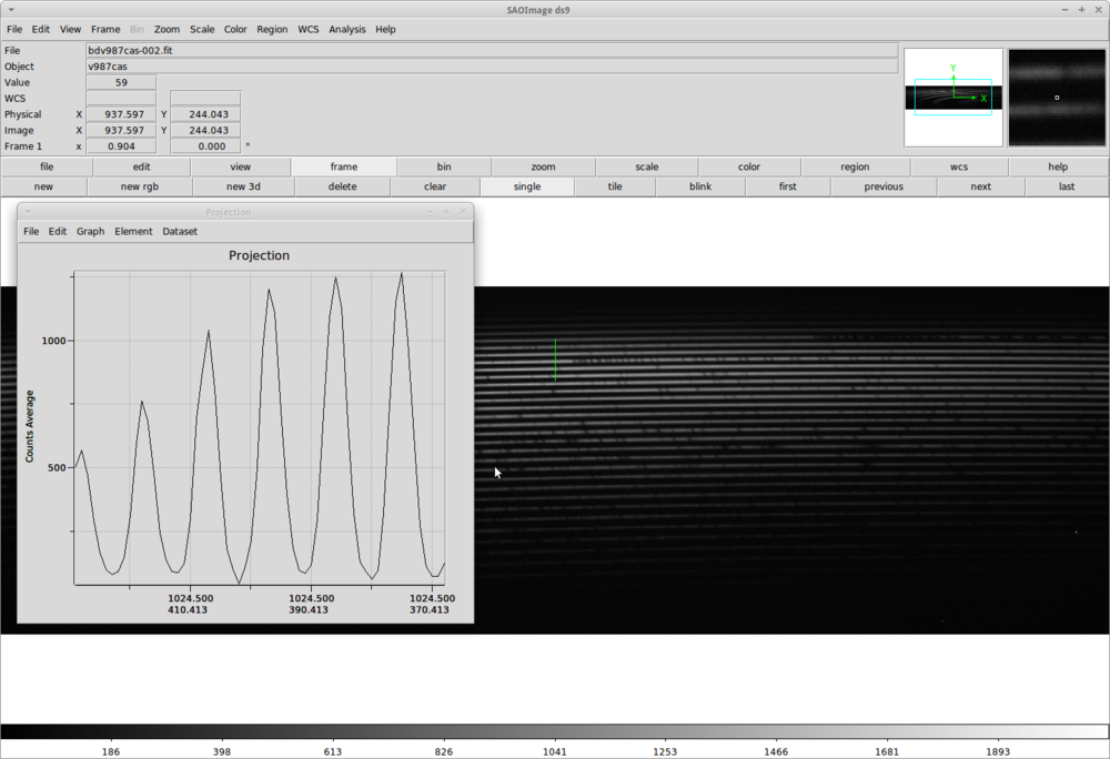
We have to meassure the width of our apertures. One way of doing this is to open an image with DS9 and from the menu use Region => Shape => Projection option and mark a line perpendicular to the spectral lines. In the popup Projection window we can read the width of the apertures.
Tracking the apertures
- Noao => imred => echelle => epar doecslit
- objects: @bdfobj.list
- apref: aperture reference spectrum(for example one of the objectum filename without the .fits)
- arcs: spectral lamp spectra(if does not accepts listfiles, you should type the different filenames separated with a comma, without the .fits)
- norders: 35
- width: 10 (the order profiles width)
- clean: yes
- trace: yes
- backgro: none
- splot: plots the final spectra(yes)
The doecslit task has basic parameters, which you can set by typing :e in the field of sparams. First run the task, then type a capital i. This will cancel the task and put you back to the xgterm window from the irafterm window. This is necessary, because, you cant change the size of the irafterm window while it is active. Enlarge the window so you can work with it comfortably, then run doecslit again.
WARNING!!! DO NOT CLOSE THE IRAFTERM WINDOW, OR IRAF WILL FREEZE!!! (at least my version of IRAF can't handle this)
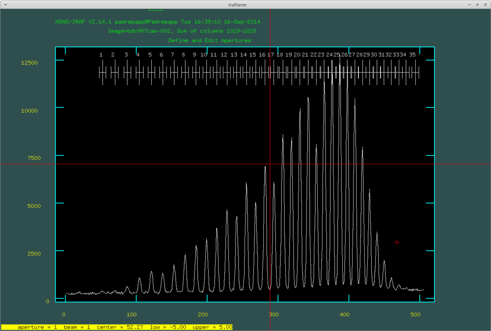
After this we can look at the apertures. We can delete undesired orders with hovering over them with the cursor and pressing d, and mark orders with m. You van define the order number with o.
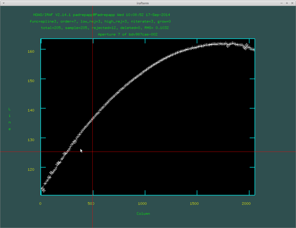
With pressing q we can move forward to the next step of the task. It will ask if we would like to fit the aperture interactively. If you accept, you can look at all the aperture fit moving forward with q and RETURN. You can delete points from the fits hovering over it your cursor and pushing d.
If we have multiple object images, and the fitting our acceptable, you can select no for the interactive question.
Wavelength calibration
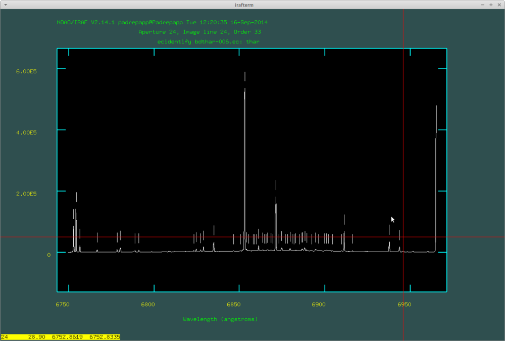
After tracking the apertures, the next step in the doecslit task is to identify the lines in the spectral lamp image. You can use the ThAr spectral maps of Balázs Csák (http://tesla.gothard.hu/~obs/.po/PO_ThAr.pdf.pdf) and Levente Kriskovics (media:tharmap.pdf), or using an online site like: http://iraf.noao.edu/specatlas/thar/thar.html
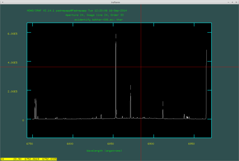
By pressing m on a line you can set its wavelength, with d you can delete if you mistyped something. With the + and - signs (on the numpad) you can move between the labeled lines. If you are ready, you can move to the next order by pushing k or to the previous order with j. If we are ready with all the orders, push y and IRAF will try to identify more lines automatically (you have to do this on every order).
After this push f to fit the dispersion function, where you can delete fitted points with d. Here are the identified lines by doecslit:
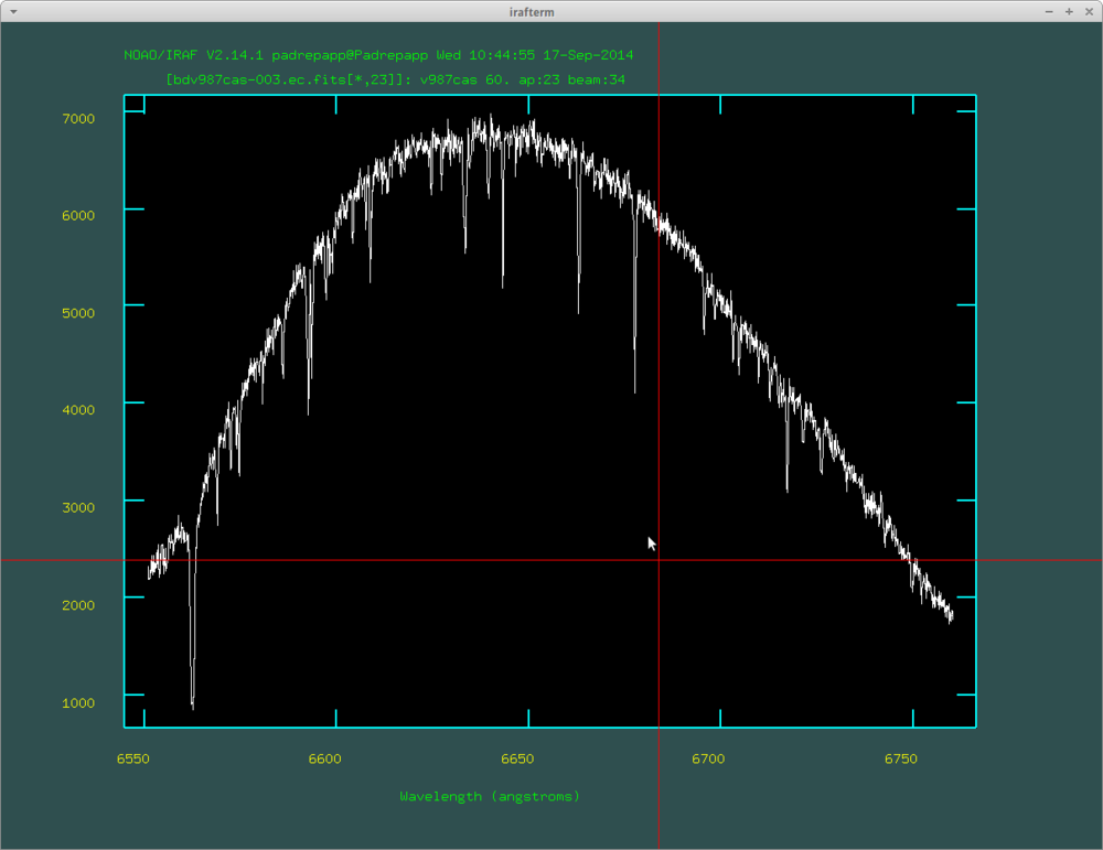
After this you will have the .ec files, you can view these with the splot task
- splot bdc987cas-007.ec.fits
You can move between the orders with the () buttons, you can zoom in an area with a, zoom out with w and a. The splot task: at the left side of the spectra you can see the H alpha line
Normalizing the Continuum
Making list files for the wavelength calibrated images:
- ls *.ec.fits > ec.list
- sed -e 's/\.ec\./\.cont\./g' ec.list > cont.list
- Noao => imred => echelle => epar continuum
- input: filename or list(@ec.list)
- output: filename or list(@cont.list)
- lines: *
- interac: yes (if we have a lot of images and it is working ok you can set no)
- low_rej: 2
- high_rej: 3
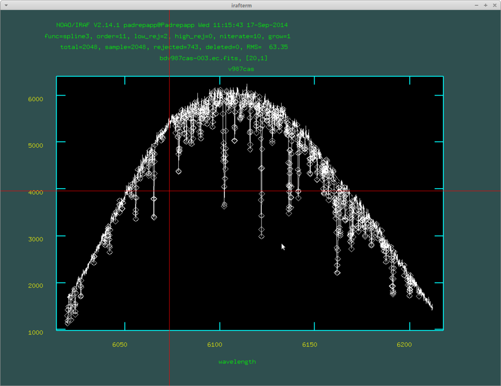
The fitted curve of the continuum task:
If you would like to exclude a bigger absoprtion region you can mark fitted regions by pressing s at the sides, and pushing f for a refit. This will be valid for the next order too, so you have to push t and f. After this we will have the continuum normalized orders.
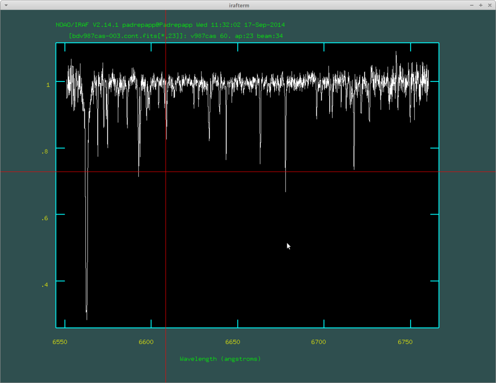
- splot bdv987cas-007.cont.fits
A continuum normalized order with the H alpha line on its left side:
Making the 1 dimensional spectra
Making list files:
- sed -e 's/\.ec\./\.normf\./g' ec.list > normf.list
- sed -e 's/\.ec\./\.ec1d\./g' ec.list > ec1d.list
- sed -e 's/\.ec\./\.normf1d\./g' ec.list > normf1d.list
- sed -e 's/\.ec\./\.cont1d\./g' ec.list > cont1d.list
Making the 1 dimensional spectra:
- sarith @ec.list / @cont.list @normf.list
- scombine @ec.list output=@ec1d.list group=images combine=sum
- scombine @normf.list output=@normf1d.list group=images combine=sum
- sarith @ec1d.list / @normf1d.list @cont1d.list
You can view the spectrum with the splot task
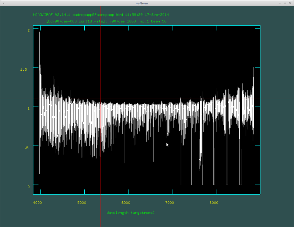
- splot bdv987cas-003.cont1d.fits
You can see that the different orders wont overlap over 7100 angstroms an that the edges are not perfect.
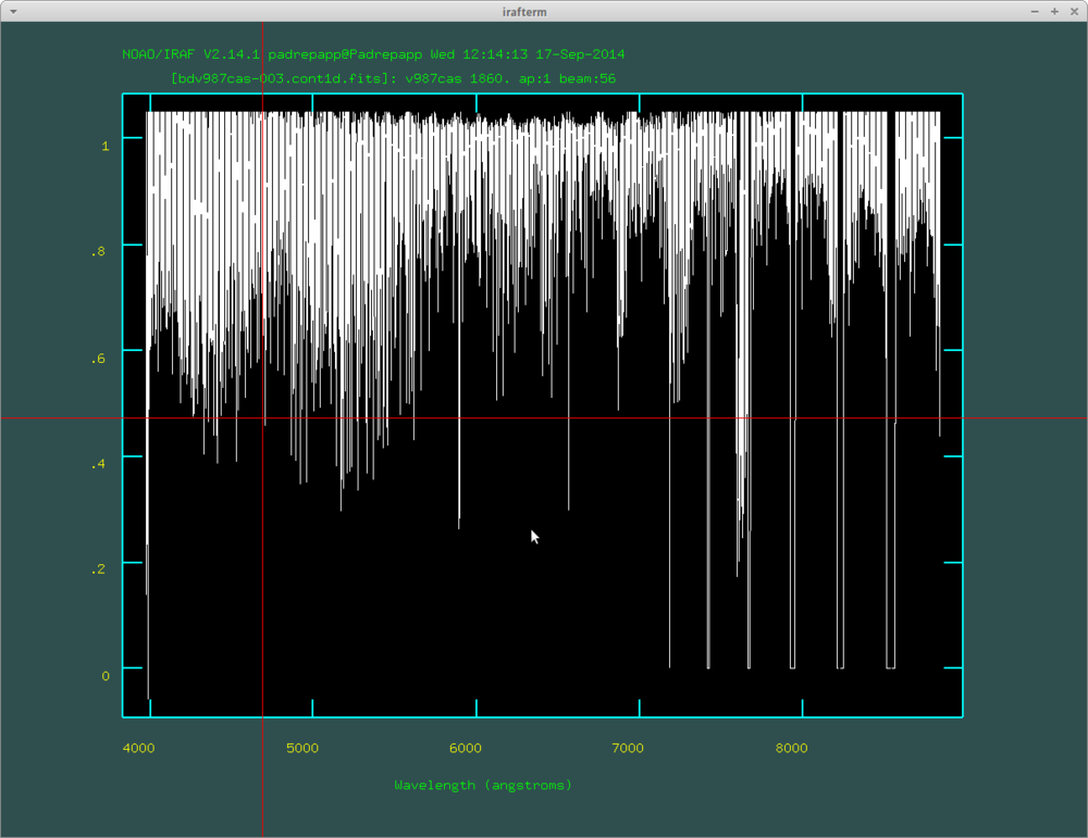
We can trim the spectra over 1 with the imreplace task.
- epar imreplace
- images: bdv987cas-003.cont1d.fits
- value: 1.05
- lower: 1.05
- upper: INDEF
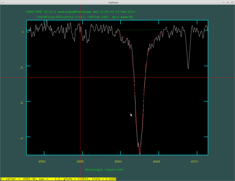
After this you can examine your spectra with the splot task. For example you can zoom in on the H alpha line by pressing a twice at the edges of the desired area, and press k two times at the edges of a line to fit a Gauss-curve, k and v for a Voigt-profile, k and l for a Lorentz-profile, you can read the equivalent width in the irafterm window's lower left corner.
The fitted Voigt-profile with the splot task
